Solving Tramp Ship Routing and Scheduling Problems

Introduction

This work was conducted within the subject TIØ4500 - Managerial Economics and Operations Research, a central part of the Master of Science In Engineering in Industrial Economics and Technology Management at the Norwegian University of Science and Technology (NTNU). The subject TIØ4500 acts as a preparatory course for the final master thesis to be written in the spring of 2023. This work and the upcoming master thesis concern Tramp Ship Routing and Scheduling Problems with Flexible Cargo Quantities and Bunker Optimization and originated through discussion with industry partners Western Bulk and Maritime Optima. As far as I know, it is the first academic study studying a Tramp Ship Routing and Scheduling problem that combines Flexible Cargo Quantities and Bunker Optimization. This article summarizes the main findings. The full report is available here.

Background

Maritime transportation is the backbone of international trade, dominating other modes of transportation in terms of total volume transported. Due to the economic effects of absolute advantages, comparative advantages, technical improvements, and economies of scale, more than 80% of the total volume traded internationally was carried on board vessels in 2019 (UNCTAD, 2022). For bulk operators in the shipping industry, a deep understanding of trade patterns and skills regarding securing transport contracts and cargo transport can make their operations financially lucrative.

In the studied problem, a dry bulk operator like Western Bulk is to deploy their fleet of hired vessels to maximize the profit for the entire fleet. To do so, they have to pick between a set of mandatory contracted cargoes and optional cargoes, potentially paying a cost for not servicing a contracted cargo. Profit is generated by the cargo transported. The variable costs include port, canal, and fuel purchase costs. As such, the dry bulk operator has to construct profit-maximizing routes and schedules for each vessel in their fleet. In the dry bulk industry, an operator can often choose the exact amount of cargo to transport from a predetermined More or Less in Owner's Option (MoLOO) interval. Thus, the operator needs to decide how much cargo to transport. As vessels may carry multiple cargoes simultaneously, the profit-maximizing amount of each cargo can be challenging to decide. Further, as the ships eventually run out of fuel, the operator must choose where to stop for fuel and the quantity of bunker (fuel) to purchase. Western Bulk relies on charting and operations managers to make such decisions. This study aims to provide these divisions with an additional tool to aid their decision-making process.

This article formulates a mathematical arc flow model that captures the complex operational environment of dry bulk operators such as Western Bulk. Results show that commercial solvers can provide optimal solutions to the arc flow formulation for smaller test instances. For larger test instances, finding an optimal solution becomes too time-consuming. A mathematical path flow model was formulated to overcome the limitations of the arc flow model. To find optimal solutions, the solver of the path flow model leverages an a priori column generation approach. This solution method generates the set of all feasible routes. Each route is then optimized to construct schedules with an optimal profit. The commercial path flow model solver selects the schedules maximizing the fleet-specific profit. The a priori column generation approach obtains optimal solutions for test instances of up to 30 cargoes, 10 vessels, and 10 bunker ports within 30 minutes.

Assumptions

The design process of the model resulted in some relatively strict assumptions. Next semester's Master Thesis will extend the model to loosen these assumptions. The following lists some of the most notable assumptions:

• Freight rates, bunker prices, and speeds are fixed for the duration of the planning horizon and are assumed to be known.
• The fleet size is fixed for the duration of the planning horizon. The contracted and mandatory may be serviced by vessels chartered in the spot market. Only vessels in the fleet may service optional spot cargoes.
• Some vessels and ports may be incompatible due to berth water depths and loading/discharging gear restrictions.
• Cargoes are uncoupled such that there are no restrictions on the order of how cargo types are transported. In real life, a vessel's cargo holds must be cleaned at a cost after transporting cement, or the vessel is limited to transporting similarly "dirty" cargoes. Dirty cargoes are not modeled in this research.
• Vessels are not allowed to fill bunker and load/discharge cargo concurrently.

Solution Methods

To model Western Bulk's operational environment, this research suggests a Mixed-Integer Linear Programming (MILP) arc flow formulation. The arc flow formulation models all of the fleet-specific constraints and the vessel-specific constraints together. Commercial solvers such as Gurobi are capable of solving such models to optimality. However, as the instance size grows, the solution time grows exponentially. The largest instance that the solver of the arc flow formulation was capable of solving within one hour consisted of 9 cargoes, two vessels, and four bunker nodes. The full arc flow formulation is presented at the end of this article

A Dantzig-Wolfe decomposition was applied to generate a path flow formulation of the original model so the limitations of the arc flow formulation could be overcome. The path flow formulation is considerably smaller than the arc flow formulation, as there are only two sets of constraints that are fleet-specific in the original arc flow model. The rest are vessel-specific and may be solved independently. Let a route be defined as a consecutive sequence of nodes a vessel will visit, e.g., {0, 23, 5, 15, 1, 11, 30}. Such a route consists of an artificial origin and destination node and potentially bunker option nodes, pickup nodes, and delivery nodes. Let a schedule be a route in which the optimal cargo to transport and the optimal bunker to purchase have been decided to optimize the vessel-specific schedule profit. Given all such optimal schedules and their corresponding profits, solving the path flow formulation yields the optimal assignments of schedules to the fleet of vessels that maximize the fleet-specific profit.

The solution method of the path flow formulation is referred to as a priori column generation and can be summarized as follows:

1. Generate all feasible routes for every vessel in the fleet
2. Optimize every route to generate their corresponding schedule with an optimal vessel-specific schedule profit.
3. Solve the path flow formulation to assign the best combination of schedules to the fleet of vessels.

The a priori column generation approach solved instances of 30 cargoes, 10 vessels, and 10 bunker ports within 30 minutes.

‍

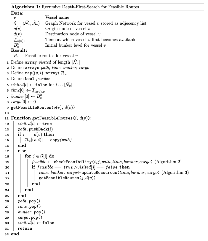
Route Generation

All feasible routes for each vessel were generated by performing a recursive Depth-First-Search of every vessel graph. In line 19, the algorithm checks for feasibility when considering a potential move to a new node. If vessel-specific constraints such as the ones that model the cargo balance, the bunker balance, or the time balance are broken, the algorithm skips to the next node. If a new node is feasible, the algorithm updates the time, bunker, and cargo resources to reflect correct values at the next node, as shown in line 21. The algorithm recursively calls itself in line 22.

‍

Schedule Generation

A Linear Programming (LP) Problem must be solved to generate the optimal schedules for each route. It consists of all of the vessel-specific constraints. As the route is given, and there are no fleet-specific constraints, all binary variables in the original arc flow formulation are excluded. Thus, the vessel schedule optimization problem is an LP problem that can be solved in polynomial time. In contrast, the original MILP arc flow formulation is NP-Hard. As such, it is possible to solve a lot of schedule optimization problems in a shorter amount of time than one would spend solving a similar path flow formulation instance. The full formulation of the schedule generation is not presented in this article but is available in the report.

Path Flow Formulation

Let ${\mathcal{R}}_v$ be a feasible sequence of node visits for vessel $v$ comprising a route.  ${\mathcal{R}}_v$ denotes the set of all feasible routes for vessel $v$. For each feasible route ${\mathcal{R}}_v$ for vessel $v$, the optimal schedule must be found. Each such schedule is associated with an optimal vessel-specific profit, denoted $P_{sv}$. Let ${\mathcal{S}}_v$ be the set of optimal schedules for vessel $v$ derived from transporting the optimal amount of cargo and purchasing the optimal amount of bunker.  Further, let the sets $\mathcal{V}$, $\mathcal{N}$, ${\mathcal{N}}^C$, and ${\mathcal{N}}^O$ denote the set of vessels, cargo-related nodes, contracted cargoes, and optional spot cargoes, respectively. As in the arc flow model, $C_i^S$ denotes the cost of servicing the cargo at pickup node $i$ with a spot ship. A new parameter, $A_{isv}$, is introduced and set equal to 1 if vessel $v$ carries cargo $i$ in schedule $s$, and 0 otherwise. The variable $x_{sv}$ defines a binary schedule variable equal to 1 if vessel $v$ is chosen to sail schedule $s$, and 0 otherwise. Finally, the binary variables $y_i\in {\mathcal{N}}^O$ and $z_i\in {\mathcal{N}}^C$ denote whether or not a spot cargo is serviced and whether or not a spot ship is used to service a Contract of Affreightment (CoA) cargo, respectively. Tables 1-3 summarize the notation used in the path flow formulation.

‍

‍

A new set of constraints must be included to ensure that each ship is assigned exactly one schedule. The Objective Function (1) and Constraints (2)-(6) present the path flow reformulation to the arc flow model presented.

$$\begin{array}{rlr}\text{(1)}& max& \sum _{v\in \mathcal{V}}\sum _{s\in {\mathcal{S}}_v}{P}_{sv}{x}_{sv}-\sum _{i\in {\mathcal{N}}^C}{C}_i^S{z}_i\text{s.t.}& & \\ \text{(2)}& & \sum _{v\in \mathcal{V}}\sum _{s\in {\mathcal{S}}_v}{A}_{isv}{x}_{sv}+z_i=1& & i\in {\mathcal{N}}^C\text{(3)}& & \sum _{v\in \mathcal{V}}\sum _{s\in {\mathcal{S}}_v}{A}_{isv}{x}_{sv}-y_i=0& & i\in {\mathcal{N}}^O\text{(4)}& & \sum _{s\in {\mathcal{S}}_v}{x}_{sv}=1& & v\in \mathcal{V}\text{(5)}& & x_{sv}\in \{0,1\}& & s\in {\mathcal{S}}_v,v\in \mathcal{V}\end{array}$$

The Objective Function (1) maximizes the fleet profit, which consists of the vessel-specific profit less the cost of hiring a spot ship to service a CoA cargo. Constraints (2) state that each contracted cargo is either transported by a vessel in the fleet or by a spot ship. Constraints (3) specify that optional cargoes may be serviced by a vessel in the fleet. Constraints (4) ensure that each vessel is assigned exactly one route. Finally, Constraints (5) define the domains of the binary schedule assignment variables.

Test Instances and Results

Tables 4 and 6 summarize relevant characteristics of the models built from the generated test instances. Tables 5 and 7 display relevant results from solving the models constructed from the same test instances. In all tables, the Instance Class columns denote the classes of generated test instances, specifying the number of cargoes, vessels, and bunker nodes. Every class consists of five randomly generated test instances. The number of spot cargoes is twice that of CoA cargoes, and the More or Less in Owner's Option (MoLOO) flexibility limits were set to $\pm$ 10%. The Size columns signify the size of the test instances classes.

In Table 4, the CPU_AF column states the solution times of the arc flow model in seconds averaged over the test instances in each class. The N_Var, N_Bin, and N_Constr columns display the average number of variables, binary variables, and constraints, respectively. Finally, the PH column gives the average number of days in the planning horizon for each test instance class. As the duration of the planning horizon is set to the largest randomly generated delivery node end-time of a test instance, each test instance has a different planning horizon. The column Solved in Table 5 shows the number of test instances within each class that were solved to optimality for the arc flow model within one hour. The BestBound_AF column displays the best dual bound found when solving the arc flow model, averaged over the test instances in each class. Similarly, the ObjVals_AF column states the best primal bounds. The Gap column shows the average percentage difference between the best primal and dual bounds.

‍

‍

‍

In Table 6, columns CPU_RG, CPU_SG and CPU_PF display the average run time in seconds for route generation, schedule generation, and solving the path flow model, respectively. The CPU_aPCG column shows the total duration of the aPCG approach, including route generation, schedule generation, and setting up and solving the path flow model. The values are displayed in seconds and averaged over the generated test instances for each class. Experiments show that setting up the path flow model is relatively slow. Finally, column N_R reports the average number of routes generated by the different classes of test instances.

In Table 7, the Solved column shows the number of test instances within each class that were solved to optimality by the aPCG approach within one hour. The N_SS and N_SC columns state the number of spot ships used and the number of spot cargoes transported in the optimal solution. Their values are averaged over the test instances in each class. Further, the ObjVal_aPCG column states the optimal solution found by the aPCG approach, averaged over the test instances in each class. Thus, if Table 7 included a Gap column, its values would all equate to zero. Finally, the $\mathrm{\Delta }$ column reports the average percentage improvements of the optimal objective value found when solving the path flow model compared to the best objective value found when solving the arc flow model.

‍

‍

‍

‍

The Arc Flow Formulation

Tables 8 - 10 provide a summary of the sets, parameters, and variables introduced in this section, respectively.

‍

‍

‍

$$\begin{array}{}\text{(6)}& \begin{array}{rl}max& \stackrel{\text{Freight Rate}\times \text{Quantity}}{\overbrace{\sum _{v\in \mathcal{V}}\sum _{i\in {\mathcal{N}}^P}{R}_i{q}_{iv}}}-\stackrel{\text{Sailing Cost}}{\overbrace{\sum _{v\in \mathcal{V}}\sum _{(i,j)\in {\hat{\mathcal{A}}}_v}{C}_{ijv}{x}_{ijv}}}-\stackrel{\text{Spot Ship Cost}}{\overbrace{\sum _{i\in {\mathcal{N}}^C}{C}_i^S{z}_i}}\\ & -\underset{\text{Bunker Cost}}{\underbrace{\sum _{v\in \mathcal{V}}\sum _{i\in {\mathcal{B}}_v}{P}_i{b}_{iv}}}+\underset{\text{Cost/Value of Surfeit/Excess Bunker}}{\underbrace{\sum _{v\in \mathcal{V}}P\cdot (l_{d(v)v}^B-B_v^0)}}\\ \text{S.T.}& \end{array}\end{array}$$

‍
 \begin{align}
   \sum_{v \in \mathcal{V}} \sum_{j \in \hat{\mathcal{N}}_v} x_{ijv} + z_{i} = 1 && i \in \mathcal{N}^C  \label{eq-contract-cargo}\tag{7}\
   \sum_{v \in \mathcal{V}}  \sum_{j \in \hat{\mathcal{N}}_v} x_{ijv} - y_{i} = 0 && i \in \mathcal{N}^O \label{eq-spot-cargo}\tag{8}\
   \sum_{j \in \hat{\mathcal{N}}_{v} } x_{o(v)jv} = 1 && v \in \mathcal{V} \label{eq-start-voyage}\tag{9}\
   \sum_{j \in \hat{\mathcal{N}}_v} x_{ijv} - \sum_{j \in \hat{\mathcal{N}}_v} x_{jiv} = 0 && v \in \mathcal{V}, i \in \hat{\mathcal{N}}_v \setminus \{ o(v), d(v)  \} \label{eq-voyage-flow}\tag{10}\
   \sum_{i \in \hat{\mathcal{N}}_{v} }  x_{i d(v) v} = 1 && v \in \mathcal{V} \label{eq-end-voyage}\tag{11}\
   \sum_{j \in \hat{\mathcal{N}}_v} x_{ijv} - \sum_{j \in \hat{\mathcal{N}}_v} x_{N+i, jv} = 0 && v \in \mathcal{V}, i \in \mathcal{N}^P_v \label{eq-service-both-nodes} \tag{12}\
   x_{ijv}\left(t_{iv} + T^{Q}_{iv} q_{iv} + T^{S}_{ijv} - t_{jv}\right) \leq 0 && v \in \mathcal{V}, (i, j) \in \hat{\mathcal{A}}_v  \label{eq-pickup-time-balance}\tag{13}\
                                                                                 && | i \in \mathcal{N}^P_v \nonumber\[1em]
   x_{ijv}\left(t_{iv} + T^{Q}_{iv} q_{i-N,v} + T^{S}_{ijv} - t_{jv}\right) \leq 0 && v \in \mathcal{V}, (i, j) \in \hat{\mathcal{A}}_v  \label{eq-delivery-time-balance}\tag{14}\
                                                                                 && | i \in \mathcal{N}^D_v  \nonumber\[1em]
   x_{ijv}\left(t_{iv} + T^{S}_{ijv} - t_{jv} \right) \leq 0 && v \in \mathcal{V}, (i, j) \in \hat{\mathcal{A}}_v  \label{eq-bunker-time-balance}\tag{15}\
                                                                                 && | i \notin \mathcal{N}^P_v \wedge i \notin \mathcal{N}^D_v \nonumber\[1em]
   t_{iv} + T^{Q}_{iv} q_{iv} + T^{S}_{i,N + i,v} - t_{N+i,v}  \leq 0 && v \in \mathcal{V}, i \in \mathcal{N}^{P}_{v} \label{eq-node-precedence}\tag{16}\
   \underline{T}_{iv} \leq t_{iv} \leq \overline{T}_{iv} && v \in \mathcal{V}, i \in \hat{\mathcal{N}}_v \label{eq-time-limits} \tag{17}\
   x_{{ijv}}\left(l^{C}_{iv} + q_{jv} - l^{C}_{jv}\right)  = 0 && v \in \mathcal{V}, (i,j) \in \hat{\mathcal{A}}_v  \label{eq-pickup-cargo-balance}\tag{18}\
                                                                                 && | j \in \mathcal{N}^P_v \nonumber \[1em]
   x_{{i,N+j,v}}\left(l^{C}_{iv} - q_{jv} - l^{C}_{N+j,v}\right) = 0 && v \in \mathcal{V}, (i, N+j) \in \hat{\mathcal{A}}_v  \label{eq-delivery-cargo-balance}\tag{19}\
                                                                                 && | j \in \mathcal{N}^P_v \nonumber\[1em]
   x_{{ijv}}\left(l^{C}_{iv} - l^{C}_{jv}\right)= 0 && v \in \mathcal{V}, (i,j) \in \hat{\mathcal{A}}_v  \label{eq-bunker-cargo-balance}\tag{20}\
                                                                                 &&  | j \in \mathcal{B}_v \nonumber\[1em]
   l^C_{o(v),v} = 0 && v \in \mathcal{V} \label{eq-initial-cargo}\tag{21}\
   q_{iv} \leq l^{C}_{iv} \leq \sum_{j \in \hat{\mathcal{N}}_v} K_v x_{ijv} && v \in \mathcal{V}, i \in \mathcal{N}^P_v \label{eq-load-pickup}\tag{22}\
   0 \leq l^{C}_{N+i, v} \leq \sum_{j \in \hat{\mathcal{N}}_v} \left(K_v - q_{iv}\right)  x_{N+i, jv}  && v \in \mathcal{V}, i \in \mathcal{N}^P_v \label{eq-load-discharge}\tag{23}\
   \sum_{j \in \hat{\mathcal{N}}_v} \underline{Q}_i x_{ijv} \leq q_{iv} \leq \sum_{j \in \hat{\mathcal{N}}_v}  \overline{Q}_i x_{ijv} &&  v \in \mathcal{V}, i \in \mathcal{N}^P_v \label{eq-cargo-carry-limits} \tag{24}\
   x_{ijv}\left(l^{B}_{iv} - B^S_{ijv} - B^P_{jv} T^{Q}_{jv}q_{jv} - l^B_{jv} \right) = 0  &&v \in \mathcal{V}, (i, j) \in \hat{\mathcal{A}}_v \label{eq-bunker-pickup-balance}\tag{25}\
                                                                                 && | j \in \mathcal{N}^P_v \nonumber \[1em]
   x_{ijv}\left(l^{B}_{iv} - B^S_{ijv} - B^P_{iv} T^{Q}_{jv}q_{j-N,v} - l^B_{jv} \right) =  0  &&v \in \mathcal{V}, (i, j) \in \hat{\mathcal{A}}_v \label{eq-bunker-delivery-balance}\tag{26}\
                                                                                 && | j \in \mathcal{N}^D_v \nonumber \[1em]
   x_{ijv}\left(l^{B}_{iv} - B^S_{ijv} + b_{jv} - l^B_{jv}\right) = 0  &&v \in \mathcal{V}, (i, j) \in \hat{\mathcal{A}}_v \label{eq-bunker-bunker-balance}\tag{27}\
                                                                                 && | j \in \mathcal{B}_v \nonumber \[1em]
   x_{ijv}\left(l^{B}_{iv} - B^S_{ijv} - l^B_{jv} \right) = 0  &&v \in \mathcal{V}, (i, j) \in \hat{\mathcal{A}}_v  \label{eq-bunker-od-balance}\tag{28}\
                                                                                 &&| j \in \{d(v)\}\nonumber\[1em]
   l^{B}_{o(v)v} = B^0_v  &&v \in \mathcal{V} \label{eq-bunker-start} \tag{29}\

   \sum_{j \in \hat{\mathcal{N}}_v}  \left(\underline{B}_v +  B^S_{ijv} + B^P_{jv} T^{Q}_{jv} q_{jv}    \right) x_{ijv}  \leq  l^B_{iv} \leq \overline{B}_v \sum_{j \in \hat{\mathcal{N}}_v} x_{ijv} &&v \in \mathcal{V}, i \in \hat{\mathcal{N}}_v \label{eq-bunker-cargo-limits}\tag{30}\
   b_{iv} \leq \left(  \overline{B}_v -  \underline{B}_v  \right) \sum_{j \in \hat{\mathcal{N}}_v} x_{ijv} && v \in \mathcal{V}, i \in \mathcal{B}_v \label{eq-bunker-load-limits}    \tag{31}\
   x_{ijv} \in \{0,1\} && v \in \mathcal{V}, (i, j) \in \hat{\mathcal{A}}_v \label{eq-take-cargo}\tag{32}\
   y_i \in \{0,1\} && i \in \mathcal{N}^O \label{eq-take-spot}\tag{33}\
   z_i \in \{0,1\}&& i \in \mathcal{N}^C\label{eq-take-spot-ship}\tag{34}\
   t_{iv} \in {+} && v \in \mathcal{V}, i \in \hat{\mathcal{N}}_v \label{eq-positive-time}\tag{35}\
   q_{iv} \in ℝ^{+} && v \in \mathcal{V}, i \in \mathcal{N}^{P}_v \label{eq-positive-moloo}\tag{36}\
   b_{iv} \in ℝ^{+} && v \in \mathcal{V}, i \in \mathcal{B} \label{eq-positive-bunker-purchase}\tag{37}\
   l^{C}_{iv} ℝ^{+} && v \in \mathcal{V}, i \in \hat{\mathcal{N}}_v \label{eq-positive-cargo-load}\tag{38}\
   l^{B}_{iv} \in ℝ^{+} && v \in \mathcal{V}, i \in \hat{\mathcal{N}}_v \label{eq-positive-bunker-load}\tag{39}
 \end{align}

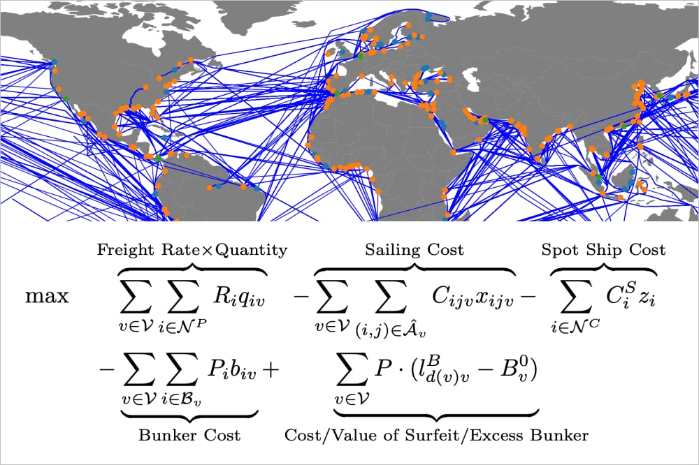
The objective function (1) aims to maximize the total profit for the deployed fleet. The first term specifies the revenue generated for both contracted and optional cargoes as a function of the quantity transported. The second term specifies the variable voyage costs associated with servicing a cargo. The final term on the first line represents the charter costs associated with servicing a contracted cargo with a spot ship. Together, the first line describes the objective presented by Christiansen et al. (2014). The fourth term describes the cost associated with purchasing bunker, and the fifth term models the value of the bonus bunker remaining at the destination node. Note that if the bunker level at the destination is higher than at the origin, this term will positively contribute to the objective. Conversely, a lower bunker level at the destination than at the origin yields a negative contribution.

Constraints (7)-(12) denote the network flow constraints of the arc flow formulation. Constraints (7) ensure that all contract cargoes are transported by a vessel in the predefined fleet or by a spot ship. In contrast, Constraints (8) state that all spot cargoes must be transported by a vessel in the predefined fleet or not at all. Constraints (9) ensure that all vessels begin a schedule from their origin node and travel to a pickup node, a bunker option node, or directly to their destination node. Constraints (10) denote the flow conservation, while Constraints (11) ensure that all vessels travel to their destination node, either from a delivery node, a bunker option node, or their origin node. Together, Constraints (9) - (11) describe the flow on the sailing route used by vessel $v$. For each cargo $i$ and vessel $v$, Constraints (12) ensure that the same vessel services both the pickup and the cargo's corresponding delivery node.

Constraints (13)-(17) handle the temporal aspects of the problem. Constraints (13) state that if vessel $v$ travels directly from node $i$ to node $j$, then, the time at which a vessel $v$ begins loading of cargo in node $j$ must be greater than or equal to the time at which the vessel began loading of cargo in node $i$ plus the sum of a quantity dependent loading time at node $i$ and the sailing time from node $i$ to node $j$. Similarly, Constraints (14) specify the time progression for delivery nodes if vessel $v$ travel directly from node $i$ to node $j$. Note, however, that the cargo quantity variable $q_{iv}$ is only defined for pickup nodes, and as such the term that specifies the variable discharge time uses a different index. Constraints (15) describe a similar time flow for origin, bunker, and destination nodes as there is no cargo loading or discharging at these nodes. Constraints (16) are precedence constraints forcing the pickup node to be serviced before its corresponding delivery node. The inequality signs of Constraints (13) - (16) give vessels the option to wait before beginning their service at node $j$. Finally, Constraints (17) are the time window constraints of within a vessel must begin their service at node $i$.

Constraints (18)-(24) describe the restrictions related to the handling of the cargo transported. Constraints (18) state that if a vessel $v$ travels directly from node $i$ to a pickup node $j$, then, the cargo load on board the vessel just after completing service at node $i$ plus the cargo loaded at node $j$ must be equal to the cargo level on board the vessel just after completing service at node $j$. Constraints (19) specify a similar cargo flow if vessel $v$ travels directly from node $i$ to delivery node $N+j$. Further, Constraints (20) enforce that if a vessel $v$ travels to a bunker node $j$, then the cargo load on board the vessel stays the same as there is no cargo loading or discharging at bunker nodes. Note that the equality sign in Constraints (18) - (20) ensure that no cargo is misplaced during the shipment. Constraints (22) describe the cargo load capacity restrictions at pickup nodes, i.e., that the cargo loaded by vessel $v$ at pickup node $i$ must be less or equal to the cargo load on board just after the vessel completes its service of node $i$ which must be less or equal to the total cargo carrying capacity of the vessel. Constraints (23) specify the cargo discharge capacity restrictions at delivery nodes, i.e., that the cargo load on board vessel $v$ just after completing its service at delivery node $N+i$ must be greater or equal to zero and less than or equal to the cargo load capacity of the vessel less the cargo loaded at pickup node $i$. Finally, Constraints (24) ensure that the cargo loaded at pickup port $i$ is within the minimum and maximum cargo load limits. The summations in Constraints (22), (23), and (24) are introduced to strengthen the formulation of the model by enforcing only one of the $x_{ijv}$ variables involved in the summation to be non-zero.

Constraints (25) - (31) describe the bunker constraints of the model. Constraints (25) state that if vessel $v$ travels directly from node $i$ to pickup node $j$, then, the bunker load on board just after completing service at node $i$ less the bunker consumption of sailing from node $i$ to node $j$ less the bunker consumed while loading at node $j$ must be equal to the bunker load on board just after completing service at node $j$. Constraints (26) specify the same balance for the delivery nodes $j$, using the similar indexing scheme as before. Constraints (27) specify the bunker load balance for bunker nodes $j$ at which there is no cargo handling. There is, however, bunker loading at node $j$ which is added to the bunker load balance. Constraints (28) describe the bunker load balance during travel to the destination node as there is no bunkering nor bunker consumption in port. The quality signs in (25) - (28) ensure that no bunker is lost during travel. Constraints (29) specify the bunker level on board vessel $v$ at the beginning of the planning period. Constraints (30) state the bunker load on board vessel $v$ just after completing its service at node $i$ must be greater than or equal to the minimum bunker level of the vessel plus the bunker consumed during sailing and cargo handling in node $j$ and less than or equal to the total bunker capacity of the vessel. Constraints (31) ensure that the bunker purchased by vessel $v$ at bunker node $i$ is less than or equal to the difference between the minimum and maximum bunker load capacity. The summations in (30) and (31) are again strengthening the formulation of the model, enforcing only one of the $x_{ijv}$ variables involved in the summation to be non-zero.

Finally, Constraints (32) - (39) specify the variables' domains.  The $x_{ijv}$ variables in Constraints (32) are binary as they specify whether a vessel $v$ travels directly from node $i$ to node $j$, or not. The $y_i$ variables in Constraints (33) are binary as they indicate whether a spot cargo is serviced, or not. The $z_i$ variables in Constraints (34) are binary as they state whether a spot ship is used to transport a contracted cargo or not. The remaining variables specified by Constraints (35)-(39) can take fractional values and are required to be non-negative. Constraints (35) state that the time variables $t_{iv}$ can never take on values from before the planning period begins. Constraints (36) denote that a vessel $v$ may never transport negative cargo from node $i$. Constraints (37) specify that a vessel $v$ may never purchase a negative amount of bunker at bunker node $i$. Constraints (38) ensure that a vessel $v$ may never have a negative cargo load on board. Finally, Constraints (39) state that there may never be a negative amount of bunker on board vessel $v$ at node $i$.