I wrote my master's thesis in the spring of 2023. It concludes my Master of science in Industrial Economics and Technology Management at the Norwegian University of Science and Technology (NTNU).
The maritime transport industry plays a crucial role in the global economy, with over 11 billion metric tonnes of goods traded by sea in 2019. Within this complex and diverse industry, dry bulk operators like Western Bulk exploit regional arbitrage opportunities when offering cargo transport services. This research focuses on a specific challenge faced by dry bulk operators, such as Western Bulk, known as the Tramp Ship Routing and Scheduling Problem with Bunker Optimization (TSRSPBO). This problem aims to maximize the overall profit of a fleet of vessels by selecting the most profitable cargoes from a pool of available options. The formulation of this problem incorporates flexible cargo limits (MOLOO) and integrated bunker optimization. Additionally, the study addresses the regional allocation of vessels and fleet repositioning. Consequently, a solution to this problem must determine the appropriate cargo quantities to transport, make routing and scheduling decisions regarding cargo and bunker ports, select the optimal bunker quantity to procure from each port and pinpoint the regions in which vessels should be located at the end of the planning period. In my thesis, I modeled the studied TSRSPBO as a two-stage stochastic optimization problem, where routing and bunkering decisions are solved in the first-stage problem, and the recourse cost of fleet repositioning is considered in the second-stage.
The industry partner of this thesis, Western Bulk, operates a long-term fleet of 30 vessels. To solve test instances of this size, a Adaptive Large Neighborhood Search (ALNS) heuristic is proposed. Results show that the iterative heuristic finds near-optimal solutions for small- and medium-sized test instances. Furthermore, the heuristic successfully solves test instances of 120 cargoes, 30 vessels, and ten bunker ports in under one hour.
A full mathematical optimization model is presented at the end of this blog post.
Solution Approach
Figure 1 provides a high-level overview of the implemented ALNS heuristic. The algorithm begins by constructing an initial solution. Next, a combination of destroy and repair operators are applied in sequence to generate a candidate solution \(x^{cand}\). To explore other feasible solutions in the local neighborhood of \(x^{cand}\), local search is applied to the \(x^{cand}\) solution. The sequence of destroy and repair operators, as well as the local search operators, aims to find solutions to the first-stage problem.
After the local search operators are applied to the \(x^{cand}\) solution, the expected second-stage recourse cost of repositioning the fleet is deducted from the profit of \(x^{cand}\) discovered during the first-stage solution search. The cost can be calculated by solving the second-stage problem formulated which minimizes the cost of repositioning. Additionally, the Vessel Combination Problem (VCP) is solved in every \(I^{VCP}\) iteration. The VCP is solved using all the routes encountered during the ALSN procedure, and its solution replaces \(x^{cand}\). As such, the VCP is solved for a subset of all feasible routes.
Once the first-stage and the second-stage phases of the ALNS heuristic in Figure 1 have been completed, the candidate solution \(x^{cand}\) is checked to determine whether it should be accepted as the accepted solution \(x^{acc}\). The acceptance criterion of the implemented ALNS follows a simulated annealing approach. Therefore, candidate solutions may be accepted even though they are worse than the best-known solution. If a candidate solution is accepted, \(x^{acc} \leftarrow x^{cand}\), and otherwise \(x^{cand}\) is discarded. Finally, the ALNS stop criterion determines whether the heuristic should continue or return the best-found solution.
The ALNS heuristic starts by constructing an initial solution for the provided test instance. Let \(\mathcal{U}\) denote the set of cargoes not assigned to any vessel in the fleet. The construction heuristic begins by setting \(\mathcal{U} \leftarrow \mathcal{N}^P\), the set of pickup nodes. Additionally, the initial routes for each vessel are set to only include the origin and destination node, \(o(v)\) and \(d(v)\), respectively. At each iteration, a cargo, represented by the pickup and delivery node-pair \((i, i+N) | i \in \mathcal{N}^P, i+N \in \mathcal{N}^D\), is inserted into a vessel's route at the position that increases the fleet-specific profit by the most. Subsequently, \(i\) is removed from \(\mathcal{U}\). As such, the construction heuristic implements a greedy insertion criterion. the construction heuristic terminates when either \(\mathcal{U} = \emptyset\) or there are no feasible cargo insertions.
Constructing an Initial Feasible Solution
The ALNS heuristic starts by constructing an initial solution for the provided test instance. Let \(\mathcal{U}\) denote the set of cargoes not assigned to any vessel in the fleet. The construction heuristic begins by setting \(\mathcal{U} \leftarrow \mathcal{N}^P\), the set of pickup nodes. Additionally, the initial routes for each vessel are set to only include the origin and destination node, \(o(v)\) and \(d(v)\), respectively. At each iteration, a cargo, represented by the pickup and delivery node-pair \((i, i+N) | i \in \mathcal{N}^P, i+N \in \mathcal{N}^D\), is inserted into a vessel's route at the position that increases the fleet-specific profit by the most. Subsequently, \(i\) is removed from \(\mathcal{U}\). As such, the construction heuristic implements a greedy insertion criterion. the construction heuristic terminates when either \(\mathcal{U} = \emptyset\) or there are no feasible cargo insertions.
The construction heuristic must check the potential route's profitability when deciding what cargo to insert in which vessel's route in what position. Each potential route must also be checked for feasibility with regard to the time balance, cargo balance, and bunker balance constraints. Additionally, the bunker node that contributes most to a vessel's route profit must be inserted at its best position.
Table 1 illustrates the results of running the construction heuristic on an example test instance. The set \(\mathcal{B} = \{11, 12\}\) denotes bunker nodes. The origin nodes, \(o(v)\), are represented by 0, and the artificial destination nodes, \(d(v)\) are represented by 13.
Destroy Operators
Given a feasible solution, the destroy operators aim to destroy the current solution by removing cargo nodes. Subsequently, the repair operators aim to repair the destroyed solution in such a way that the resulting solution is better than the original. The three implemented destroy operators are named random removal, Shaw removal, and worst removal.
Random removal - Select at random which cargoes to remove
Shaw removal - Remove cargoes that are similar with respect to a weighted sum of distance
Worst removal - Remove the least profitable cargoes from a current solution.
Repair Operators
Repair operators aim to repair a destroyed solution by inserting cargoes in such a way that the resulting solution is more profitable than the original solution. In my thesis, I implemented a single repair operator, the regret-k repair operator. The regret-k operator can be parameterized to generate different versions of itself. The \(k\) parameter defines the preference for how greedy the repair operator should act. By using \(k=1\), the repair operator inserts the most profitable cargo at each iteration. However, for larger values of \(k\), the regret-k operator tries to look ahead, by calculating a regret score. This score is a measure of how much the global profitability of a solution might suffer by inserting the locally best cargo.
Regret-k insertion
For each cargo in \(\mathcal{U}\), for each position in each vessel's current route, calculate the marginal profit to the current solution if the cargo were to be inserted at the position in the vessel's route.
For each cargo, sort the marginal profits in descending order, and calculate the cargo's regret score.
The regret score is calculated by measuring how quickly the marginal profits for a cargo drops off as you move along the sorted list of possible cargo insertions.
A cargo with a lot of profitable insertions yield a low regret score.
A cargo with a single profitable insertion with subsequent unprofitable insertions result in a high regret score. - In other words, if the profitable cargo insertion is not performed, the repair operator will regret its decision later.
For as long as there are feasible cargo insertions, insert the cargo yielding the highest regret score.
When calculating the regret score, the \(k\) parameter signifies the number of cargo insertions to consider before calculating how quickly the marginal profits drop.
Selection of Destroy and Repair Operators
In my thesis I implemented three destroy operators, and three versions of the repair operator. However, at every iteration of the ALNS, a single destroy operator, and a single repair operator is applied to the current solution. As such, at each iteration we must select which operator to apply to the current solution. The selection mechanism is based on scoring the performance of the different operators. They are rewarded for finding better solutions, and also rewarded for exploring a different portion of the problem search space. At each iteration the operators are chosen based on roulette wheel selection according to their reward score.
Local Search
The application of subsequent destroy and repair operators allow the ALNS heuristic to jump around a lot in the search space of feasible solutions. As such, local search operators can be applied to exhaustively explore the local neighborhood for a solution. The below figure represents the feasible search space in which the ALNS heuristic aims to find the best possible solution. Each center of a circle represents a solution obtained by applying the destroy-repair operator sequence at each iteration of the ALNS heuristic. The dotted circles around each center represents the local neighborhood of a feasible solution. By applying local search operators, this area of the search space is exhaustively explored. As the entire search space might be extremely large, an exhaustive search of the entire search space is intractable. The red cross represents the best solution found by the ALNS heuristic. In contrast, the blue cross is the globally optimal solution. The figure illustrates that the ALNS heuristic is not guaranteed to find an optimal solution. However, it is expected to find high-quality solutions that are often similar to the optimal solution. Note also that the red cross found not be found unless we exhaustively explore the local neighborhood in iteration 5.
In my thesis, I implemented the CROSS-Exchange local search operator. The CROSS-exchange operator involves selecting two pairs of edges in two different routes, and exchanging them in a way that generates two new routes. Specifically, four nodes \(i,k,j,l\) are selected such that \(i\) and \(k\) belong to the same route, and \(j\) and \(l\) belong to a different route. Next, the edges \((i,i+1)\) and \((j,j+1)\) are swapped to produce edges \((i, j+1)\) and \((j, i+1)\). Similarly, edges \((k-1, k)\) and \((l-1, l)\) are also swapped to generate edges \((l-1, k)\) and \((k-1, l)\). The below figure illustrates the process.
Vessel Combination Problem (VCP)
All feasible vessel routes encountered by the ALNS heuristic are stored for the duration of the search. At every 100th iteration of the ALNS heuristic, a vessel combination problem (VCP) is solved to find the optimal combination of vessel routes given the encountered routes.
The vessel combination problem is modeled as a stochastic two-stage path flow formulation. Let \(\mathcal{R}_v\) denote the set of feasible routes for vessel \(v\), indexed by \(r\). The routes in \(\mathcal{R}_v\) for vessel \(v\) are referred to as routes. Further, let the sets \(\mathcal{V}\), \(\mathcal{N}\), \(\hat{\mathcal{N}}_v\), \(\mathcal{N}^C\), \(\mathcal{N}^O\), \(\mathcal{K}\), and \(\mathcal{S}\) denote the set of vessels, cargo-related nodes, set of nodes vessel \(v\) may visit, contracted cargoes, optional spot cargoes, regions, and scenarios, respectively.
For each route \(r \in \mathcal{R}_v\) for vessel \(v\) there is a vessel-specific profit denoted \(R_{rv}\). The \(C^S_i\) parameter denotes the cost of servicing the cargo at pickup node \(i\) with a spot ship. An additional parameter, \(A_{irv}\), is introduced and set equal to 1 if vessel \(v\) carries cargo \(i\) in the optimized route \(r\), and 0 otherwise. Let \(B_{irv}\) equal 1 if node \(i\) is the destination node in route \(r\) of vessel \(v\), and 0 otherwise. Let \(D_{ivk}\) be equal to 1 if node \(i\) is in region \(k\) for vessel \(v\), and 0 otherwise. As in the arc flow model, let \(R^K_{ks}\) denote the number of vessels to be allocated in each region, \(r\), in each scenario, \(s\). The \(C^B_{ivk}\) parameter represents the repositioning cost from node \(i\) for vessel \(v\) to region \(k\). Finally, let \(P_{s}\) denote the probability of scenario \(s\) taking place.
The variable \(x_{rv}\) defines a binary variable equal to 1 if vessel \(v\) is chosen to sail route \(r\), and 0 otherwise. Variables \(y_i \in \mathcal{N}^O\) and \(z_i \in \mathcal{N}^C\) are defined as before, denoting whether or not a spot cargo is serviced and whether or not a spot ship is used to service a Contract of Affreightment (CoA) cargo, respectively. Variable \(x^E_{iv}\) is defined to equal 1 if vessel \(v\)'s destination is node \(i\), and 0 otherwise. Finally, let the second-stage stochastic recourse variable \(x^B_{ivks}\) be equal to 1 if vessel \(v\) repositions from node \(i\) to region \(k\) in scenario \(s\), and 0 otherwise.
Tables 2 - 4 summarize the notation used in the path flow formulation.
The following presents the two-stage stochastic path flow formulation for the Tramp Ship Routing and Scheduling problem studied in my thesis.
VCP First-Stage Formulation
Objective (1) and Constraints (2) - (9) comprise the first-stage formulation. The first term in Objective (1) sums up the vessel-specific profit generated by each of the vessels in the fleet. The second term denotes the cost of hiring a spot ship to service a CoA cargo and is subtracted from the vessel-specific profit generated. Finally, the second-stage \(\mathcal{Q}(\boldsymbol{x^E})\) term representing the recourse cost of repositioning vessels in the fleet is subtracted from the vessel-specific profit. Here, \(\boldsymbol{x^E}\) denotes the collection of \(x^E_{iv}\) variables specifying whether node \(i\) is a vessel \(v\)'s destination node, or not. Constraints (2) state that each contracted cargo is either transported by a vessel in the fleet or by a spot ship. Constraints (3) specify that optional cargoes may be serviced by a vessel in the fleet. Constraints (4) ensure that each vessel is assigned exactly one route. Constraints (5) assigns the correct values to the \(x^E_{iv}\) variables such that \(x^E_{iv}\) is equal to 1 if vessel \(v\)'s destination is node \(i\), and 0 otherwise. Constraints (6) - (9) confine the binary variables to their respective domains.
VCP Second-Stage Formulation
Objective (10) and Constraints (11) - (13) define the second-stage path flow formulation of the VCP. Objective (10) minimizes the recourse cost which consists of the expected cost of repositioning vessels in the fleet aggregated across each scenario \(s \in \mathcal{S}\). Constraints (11) state that a vessel may at most reposition to one region. The \(x^E_{iv}\) variables are used on the right hand side of the expression to tighten the model formulation. Constraints (12) ensure that the number of vessels in each region \(k\) in each scenario \(s\) equals the predetermined parameter, \(R^K_{ks}\). The first term in the variable expression counts up the number of vessels ending up in each region \(k\) in each scenario \(s\) as a consequence of the first-stage solution. The second term adds the number of vessels repositioning into region \(k\) in scenario \(s\). The final term counts up the number of vessels repositioning out from region \(k\) in scenario \(s\) which is subtracted from the two previous terms. Thus, the variable expression in Constraints (12) correctly count up the number of vessels ending up in each region \(r\) in each scenario \(s\). Finally, Constraints (13) confine the \(x^B_{ivks}\) variables to their binary domain.
Results
To test the performance of the implemented ALNS heuristic, 13 different classes of test instances were generated. A class is denoted by the number of cargoes, vessels, and bunker nodes. For example, the C60V15B10 instance class contains 60 cargoes, 15 vessels, and 10 bunker nodes. For each class, five different test instances were randomly generated in each class, resulting in 65 different problems. Further, each problem was solved five times by the ALNS heuristic as the algorithm is not deterministic. As a comparison, a solution method based on exhaustively searching the problem space by generating all feasible routes was implemented and its results where compared to the ALNS. This method is denoted as the A Priori (AP) route generation solution method and is further explained in this blog post. The AP method was limited to generating columns for up to one hour, after which a solution was not considered to have been found. The ALNS heuristic was similarly run for up to 3,600 seconds, after which the best-encountered solution was returned.
Table 5 summarizes the results. The Instance Class column shows the solved classes of test instances along with their size. The ObjAP presents the objective value found by solving the test instances by the AP method. The values are averaged across the test instances and runs in each class. The TimeAP[s] column displays the averaged duration of the a priori column generation. ObjAV gives the objective value found by solving the test instances by the ALNS heuristic. The values are averaged across the five runs and test instances in each instance class. Similarly, the TimeAV[s] column shows the averaged solution time of the ALNS heuristic. The CV[%] column presents the coefficient of variation calculated across the five ALNS runs of each test instance. The values are then averaged across the test instances in each instance class. Finally, the Gap[%] column displays the averaged absolute percentage gap between the exact solution found by the AP solution method and the ALNS heuristic. The values are rounded to two decimals.
The results presented in Table 5 demonstrate the effectiveness of the different solution approaches. The AP solution method, successfully solves all small test instances optimally. However, it only achieves optimal solutions for three out of five medium-sized instances and none of the large instances. In contrast, the ALNS heuristic is capable of solving all small and medium-sized instances within an hour. Among the large instances, the ALNS heuristic solves all test instances of the C60V15B10 and C90V20B10 classes within an hour, while instances in the other large classes reach the one-hour stopping criterion.
The ALNS heuristic achieves optimal solutions for all small-sized C12V4B6 instances. For the remaining small instances, the optimality gaps are less than 0.005, which are considered negligible and rounded to zero. In the first three medium-sized classes, the ALNS reports average optimality gaps of 0.01, 0.02, and 0.01, respectively, indicating high-quality solutions. Since the AP approach fails to solve larger instances, no optimality gaps are reported for them. However, the ALNS provides solutions for all generated test instances. The CV[%] column values remain relatively low for larger instances, indicating that the ALNS heuristic produces solutions of similar high-quality across multiple runs, even for larger-sized test instances.
Furthermore, a comparison of solution times reveals interesting insights. For small-sized instances, the AP approach is advantageous, providing optimal solutions in a shorter solution time. However, for the C15V5B10, C30V5B10, and C30V10B10 classes, the ALNS delivers near-optimal solutions with significantly reduced computation times of 52%, 84%, and 83%, respectively.
Overall, when comparing the ALSN heuristic to the AP approach, it is evident that the path flow approach cannot solve optimally or even produce feasible solutions to larger instances. In contrast, the ALNS consistently produces high-quality solutions within the one-hour time limit, making it a practical operational support tool for dry bulk operators like Western Bulk, even for realistic-sized problems.
Arc Flow Formulation
The following section provides a full mathematical arc flow formulation for the studied problem, and includes more details about the vessel-specific constraints that are incorporation both in the problem definition and in the ALNS heuristic solution method.
The notation and formulation presented in this section follow the arc flow formulation of the Tramp Ship Routing and Scheduling Problem presented by Christiansen et al. (2007), the flexible cargo quantities extension formulated in Christiansen et al. (2014), and the bunker management extension devised by Vilhelmsen et al. (2014). Additional notation is introduced to present the stochastic formulation of the problem.
Let the fleet of vessels be represented by the set \(\mathcal{V}\), indexed by \(v\). Assume \(N\) cargoes are available for transport, indexed by \(i\). The sets of pickup and delivery nodes are given by \(\mathcal{N}^P = \{0, \ldots, N\}\) and \(\mathcal{N}^D = \{N + 1, \ldots, 2N\}\), respectively. These sets allow each cargo \(i\) to be represented by a pickup node \(i \in \mathcal{N}^P\) and a delivery node \(N + i \in \mathcal{N}^D\). As such, the set of all cargo-related nodes is represented as \(\mathcal{N} = \mathcal{N}^P \cup \mathcal{N}^D\). The set of pickup nodes \(\mathcal{N}^P\) is partitioned into \(\mathcal{N}^P = \mathcal{N}^C \cup \mathcal{N}^O\), where \(\mathcal{N}^C\) and \(\mathcal{N}^O\) denote the mandatory contracted and optional spot cargoes, respectively. A vessel has a node of origin \(o(v)\), a geographical position at sea or in port. It is assigned an artificial destination node \(d(v)\), which a vessel will travel to after its last planned discharge node service. Due to cargo capacity, depth, and cargo handling equipment restrictions, some vessels and nodes in \(\mathcal{N}\) may be incompatible. Thus, the set of nodes a vessel \(v\) may visit is represented as \(\mathcal{N}_v \subseteq \mathcal{N} \cup \{o(v), d(v)\}\). \((\mathcal{N}_v, \mathcal{A}_v)\) defines a base network for each vessel \(v\), where the set of arcs \(\mathcal{A}_v \subseteq \{(i, j) | i \in \mathcal{N}_v, j \in \mathcal{N}_v\}\) represents all arcs traversable by vessel \(v\) with respect to time and bunker consumption. The pickup and delivery nodes compatible with vessel \(v\) are defined as \(\mathcal{N}^P_v =\mathcal{N}^P \cap \mathcal{N}_v\) and \(\mathcal{N}^D_v = \mathcal{N}^D \cap \mathcal{N}_v\) for convenience.
The next step is extending the base network \((\mathcal{N}_v, \mathcal{A}_v)\) to allow vessel visits at bunker option nodes. Let \(\mathcal{B}\) be the set of bunker option nodes. Similarly, as for the cargo-related nodes, vessels and bunker option nodes may be incompatible. Thus, set \(\mathcal{B}_v \subseteq \mathcal{B}\) denotes the bunker option nodes that vessel \(v\) may visit. The set of base nodes \(\mathcal{N}_v\) for vessel \(v\) is extended to include the nodes in \(\mathcal{B}_v\) such that \(\hat{\mathcal{N}}_v= \mathcal{N}_v \cup \mathcal{B}_v\). Further, the set of base arcs \(\mathcal{A}_v\) is extended by adding all arcs connecting nodes in \(\mathcal{N}_v \setminus d(v)\) with nodes in \(\mathcal{B}_v\) that are traversable by vessel \(v\) with respect to time and bunker. The arcs from the destination node \(d(v)\) are excluded as the next node to visit is unknown. As such, the extended set of arcs is defined as \(\hat{\mathcal{A}}_v= \mathcal{A}_v \cup \mathcal{A}^B_v\), where \(\mathcal{A}^B_v\) is the set of arcs for vessel \(v\) connecting bunker option nodes \(\mathcal{B}_v\) to the nodes in \(\mathcal{N}_v \setminus d(v)\). The extended cargo-bunker network is thereby \((\hat{\mathcal{N}}_v, \hat{\mathcal{A}}_v)\).
Each node in the \((\hat{\mathcal{N}}_v, \hat{\mathcal{A}}_v)\) graphs is associated with a region \(k \in \mathcal{K}\). The set of scenarios is represented by \(\mathcal{S}\), indexed by \(s\).
Let \(T^{S}_{ijv}\) be the sailing time from node \(i\) to node \(j\) for a given vessel \(v\) and arc \((i, j) \in \hat{\mathcal{A}}_v\). If node \(j\) is a bunker node, a fixed time is added to \(T^S_{ijv}\), signifying the time spent bunkering. The time required to load or discharge one unit of cargo \(i\) with vessel \(v\) is defined as \(T^{Q}_{iv}\). The variable voyage cost \(C_{ijv}\) accounts for the costs of visiting node \(i\) and the sailing costs from node \(i\) to node \(j\) for vessel \(v\). It is important to note that the cost of the purchased bunker is not included in this parameter as the purchase of bunker will be modeled separately. Instead, let \(P^B_i\) denote the cost of purchasing one unit of bunker available in bunker option node \(i \in \mathcal{B}\). The bonus bunker remaining at the destination node \(d(v)\) is represented as \(\widetilde{P}\) and calculated as the mean of all available bunker node prices. The charter cost of servicing a contracted cargo \(i\) by a spot ship is denoted \(C^S_i\). Further, the bunker consumption at sea is denoted \(B^S_{ijv}\) for a vessel \(v\) traversing the arc \((i, j) \in \hat{\mathcal{A}}_v\). The bunker consumed by vessel \(v\) in node \(i\) per unit of time is represented by \(B^P_{iv}\). There is a unit revenue \(R_i\) generated for transporting cargo \(i \in \mathcal{N}^P\). For each node \(i \in \hat{\mathcal{A}}_v\) visited by vessel \(v\), there is a time window \(\left[ \underline{T}_{iv}, \overline{T}_{iv} \right]\) for the pickup and delivery time, defined by the earliest time \(\underline{T}_{iv}\) and the latest time \(\overline{T}_{iv}\) of the visit. Additionally, the bunker level on board each vessel \(v\) must be within a lower limit \(\underline{B}_v\) and an upper limit \(\overline{B}_v\) to ensure realistic and safe operation. The quantity of cargo that can be transported is flexible within interval \(\left[\underline{Q}_i, \overline{Q}_i \right]\), where \(\underline{Q}_i\) is the minimum quantity and \(\overline{Q}_i\) is the maximum quantity that must be transported if cargo \(i\) is serviced. The cargo carrying capacity of vessel \(v\) is denoted \(K_v\). Let \(A_{ik}\) be equal to 1 if node \(i\) is in region \(k\), and 0 otherwise. Let \(R^K_{ks}\) represent the number of vessels that are to be allocated in each region, \(r\), and in each scenario, \(s\). Further, let \(C^B_{d(v)k}\) represent the repositioning cost for vessel, \(v\), from the last visited node, \(d(v)\), to region \(k\). Finally, let \(P_{s}\) represent the probability of scenario \(s\).
The binary variable \(x_{ijv}\) is assigned the value 1 if vessel \(v\) traverses the arc \((i, j) \in \hat{\mathcal{A}}_v\), and 0 otherwise. The variables \(t_{iv}\) denote the time vessel \(v\) begins service at node \(i\). The cargo load on board a vessel \(v\) when it leaves node \(i\) is represented by the variable \(l^C_{iv}\). Similarly, the variable \(l^B_{iv}\) represents the bunker load on board vessel \(v\) just after completing service at node \(i\). The quantity of cargo \(i\) transported by vessel \(v\) is represented by \(q_{iv}\), and the quantity of bunker purchased by vessel \(v\) at bunker option node \(i\) is given by the variable \(b_{iv}\). To represent whether a contracted cargo is serviced by a spot ship, the binary variable \(z_i\) is assigned the value 1, or 0 otherwise. The binary variable \(y_i\) is assigned a value of 1 if the optional spot cargo \(i\) is serviced, and 0 otherwise. Let the binary variable \(r_{vk}\) be equal to 1 if vessel \(v\)'s last visited node is located in region \(k\), and 0 otherwise. Finally, let the binary stochastic second-stage variable \(x^B_{d(v)vks}\) be equal to 1 if vessel \(v\) repositions from its last visited node \(d(v)\) to region \(k\) in scenario \(s\), and 0 otherwise.
Tables 6 - 8 provide a summary of the sets, variable, and parameters introduced in this section, respectively.
Arc Flow Mathematical Model
This section provides a mathematical model of the stochastic two-stage Tramp Ship Routing and Scheduling Problem with Bunker Optimization (TSRSPBO) studied in this thesis.
\subsection{Arc Flow First-Stage Formulation} \label{sec-first-stage-arc-flow} This section provides the first-stage formulation of the two-stage TSRSPBO, including the first-stage objective function, network flow constraints, temporal constraints, cargo constraints, bunker constraints, regional constraints, and variable domain constraints.
Arc Flow Objective Function
The objective function (14) aims to maximize the total profit for the deployed fleet. The first term specifies the revenue generated for both contracted and optional cargoes as a function of the quantity transported. The second term specifies the variable voyage costs associated with servicing a cargo. The final term on the first line represents the charter costs associated with servicing a contracted cargo with a spot ship. Together, the first line describes the objective presented by Christiansen (2014). The fourth term describes the cost associated with purchasing bunker, and the fifth term models the value of the bonus bunker remaining at the destination node. Note that if the bunker level at the destination is higher than at the origin, this term will positively contribute to the objective. Conversely, a lower bunker level at the destination than at the origin yields a negative contribution. The final \(\mathcal{Q}(\boldsymbol{r})\) term denotes the second-stage recourse cost for repositioning vessels to suitable regions. The symbol \(\boldsymbol{r}\) denotes the collection of \(r_{vk}\) variables stating whether a vessel \(v\)'s last visited node is located in region \(k\), or not. The \(\mathcal{Q}(\boldsymbol{r})\) term is explained further below.
Arc Flow Network Flow Constraints
Constraints (15) ensure that all contract cargoes are transported by a vessel in the predefined fleet or by a spot ship. In contrast, Constraints (16) state that all spot cargoes must be transported by a vessel in the predefined fleet or not at all. Constraints (17) ensure that all vessels begin a voyage from their origin node and travel to a pickup node, a bunker option node, or directly to their destination node. Constraints (18) denote the flow conservation, while Constraints (19) ensure that all vessels travel to their destination node, either from a delivery node, a bunker option node, or their origin node. Together, Constraints (17) - (19) describe the flow on the sailing route used by vessel \(v\). For each cargo \(i\) and vessel \(v\), Constraints (20) ensure that the same vessel services both the pickup and the cargo’s corresponding delivery node.
Arc Flow Temporal Constraints
The above constraints handle the temporal aspects of the problem. Constraints (21) state that if vessel \(v\) travels directly from node \(i\) to node \(j\), then, the time at which a vessel \(v\) begins loading of cargo in node \(j\) must be greater than or equal to the time at which the vessel began loading of cargo in node \(i\) plus the sum of a quantity dependent loading time at node \(i\) and the sailing time from node \(i\) to node \(j\). Similarly, Constraints (22) specify the time progression for delivery nodes if vessel \(v\) travel directly from node \(i\) to node \(j\). Note, however, that the cargo quantity variable \(q_{iv}\) is only defined for pickup nodes, and as such the term that specifies the variable discharge time uses a different index. Constraints (23) describe a similar time flow for origin, bunker, and destination nodes as there is no cargo loading or discharging at these nodes. Constraints (24) are precedence constraints forcing the pickup node to be serviced before its corresponding delivery node. The inequality signs of Constraints (21) - (24) give vessels the option to wait before beginning their service at node \(j\). Finally, Constraints (25) are the time window constraints of within a vessel must begin their service at node \(i\).
Arc Flow Cargo Constraints
The constraints in this paragraph describe the restrictions related to the handling of the cargo transported. Constraints (26) state that if a vessel \(v\) travels directly from node \(i\) to a pickup node \(j\), then, the cargo load on board the vessel just after completing service at node \(i\) plus the cargo loaded at node \(j\) must be equal to the cargo level on board the vessel just after completing service at node \(j\). Constraints (27) specify a similar cargo flow if vessel \(v\) travels directly from node \(i\) to delivery node \(N + j\). Further, Constraints (28) enforce that if a vessel \(v\) travels to a bunker node \(j\), then the cargo load on board the vessel stays the same as there is no cargo loading or discharging at bunker nodes. Note that the equality sign in Constraints (26) - (28) ensure that no cargo is misplaced during the shipment. Constraints (30) describe the cargo load capacity restrictions at pickup nodes, i.e., that the cargo loaded by vessel \(v\) at pickup node \(i\) must be less or equal to the cargo load on board just after the vessel completes its service of node \(i\) which must be less or equal to the total cargo carrying capacity of the vessel. Constraints (31) specify the cargo discharge capacity restrictions at delivery nodes, i.e., that the cargo load on board vessel \(v\) just after completing its service at delivery node \(N + i\) must be greater or equal to zero and less than or equal to the cargo load capacity of the vessel less the cargo loaded at pickup node \(i\). Finally, Constraints (32) ensure that the cargo loaded at pickup port \(i\) is within the minimum and maximum cargo load limits. The summations in Constraints (30), (31), and (32) are introduced to strengthen the formulation of the model by enforcing only one of the \(x_{ijv}\) variables involved in the summation to be non-zero.
Arc Flow Bunker Constraints
Constraints (33) - (39) describe the bunker constraints of the model. Constraints (33) state that if vessel \(v\) travels directly from node \(i\) to pickup node \(j\), then, the bunker load on board just after completing service at node \(i\) less the bunker consumption of sailing from node \(i\) to node \(j\) less the bunker consumed while loading at node \(j\) must be equal to the bunker load on board just after completing service at node \(j\). Constraints (34) specify the same balance for the delivery nodes \(j\), using the similar indexing scheme as before. Constraints (35) specify the bunker load balance for bunker nodes \(j\) at which there is no cargo handling. There is, however, bunker loading at node \(j\) which is added to the bunker load balance. Constraints (36) describe the bunker load balance during travel to the destination node as there is no bunkering nor bunker consumption in port. The quality signs in (33) - (36) ensure that no bunker is lost during travel. Constraints (37) specify the bunker level on board vessel \(v\) at the beginning of the planning period. Constraints (38) state the bunker load on board vessel \(v\) just after completing its service at node \(i\) must be greater than or equal to the minimum bunker level of the vessel plus the bunker consumed during sailing and cargo handling in node \(j\) and less than or equal to the total bunker capacity of the vessel. Constraints (39) ensure that the bunker purchased by vessel \(v\) at bunker node \(i\) is less than or equal to the difference between the minimum and maximum bunker load capacity. The summations in (38) and (39) are again strengthening the formulation of the model, enforcing only one of the \(x_{ijv}\) variables involved in the summation to be non-zero.
Repositioning Constraints
Constraints (40) assign the correct values to the \(r_{vk}\) variables such that \(r_{vk}\) equals 1 if vessel \(v\)'s last visited node is located in region \(k\), and 0 otherwise. The collection of \(r_{vk}\) variables, \(\boldsymbol{r}\), is used to calculate the second-stage recourse cost.
Arc Flow Binary and Non-Negativity Constraints
The \(x_{ijv}\) variables in Constraints (41) are binary as they specify whether a vessel \(v\) travels directly from node \(i\) to node \(j\), or not. The \(y_i\) variables in Constraints (42) are binary as they indicate whether a spot cargo is serviced, or not. The \(z_i\) variables in Constraints (43) are binary as they state whether a spot ship is used to transport a contracted cargo or not. The remaining variables specified by Constraints (44) - (48) can take fractional values and are required to be non-negative. Constraints (44) state that the time variables \(t_{iv}\) can never take on values from before the planning period begins. Constraints (45) denote that a vessel \(v\) may never transport negative cargo from node \(i\). Constraints (46) specify that a vessel \(v\) may never purchase a negative amount of bunker at bunker node \(i\). Constraints (47) ensure that a vessel \(v\) may never have a negative cargo load on board. Constraints (48) state that there may never be a negative amount of bunker on board vessel \(v\) at node \(i\). Finally, Constraints (49) confine the \(r_{vk}\) variables to be binary as they are designed to equal 1 if vessel \(v\)’s last visited node is located in region \(k\), and 0 otherwise.
Arc Flow Second-Stage Formulation
Objective (50) and Constraints (51) - (53) represent the stochastic second-stage recourse cost problem denoted by \(\mathcal{Q}(\boldsymbol{r})\). Objective (50) minimizes the expected cost of repositioning vessels from their last visited node to the region they are to be allocated in aggregated over each scenario \(s \in \mathcal{S}\). Constraints (51) state that a vessel \(v\) may only reposition to at most one region in each scenario \(s\). Constraints (52) ensure that the number of vessels in each region \(k\) in each scenario \(s\) equals the predetermined parameter, \(R^K_{ks}\). The first term in the variable expression counts up the number of vessels ending up in each region \(k\) in each scenario \(s\) as a consequence of the first-stage solution. The second term adds the number of vessels repositioning into region \(k\) in scenario \(s\). The final term counts up the number of vessels repositioning out from region \(k\) in scenario \(s\) which is subtracted from the two previous terms. Thus, the variable expression in Constraints (52) correctly count up the number of vessels ending up in each region \(r\) in each scenario \(s\). Finally, Constraints (53) confine the \(x_{d(v)vks}\) variables to their binary domain.