Exploratory Data Analysis of Bunker Prices
Introduction
Commercial shipping is the backbone of international trade. In terms of tonne-miles maritime transport makes up by far the largest share of total global transport. In 2015 maritime transportation represented 71% of total transport [1].
While shipping is a carbon efficient mode of transportation [2], concerns have been raised about the greenhouse gas emissions associated with the industry. The industry combusts regularly close to 8% of oil produced annually and in 2012 made up 2.4% of global emissions [3].
These emissions are mainly a result of the bunker (fuel) used to propel the vessels. As such, the International Maritime Organization (IMO) is playing an increasingly important role of regulating the greenhouse gas emissions from the industry. Some emission reduction targets include:
- By 2025 new ships built must be 30% more energy efficient than those built in 2014
- At least a 40% reduction in carbon intensity by 2030 and pursuing efforts towards a 70% reduction by 2050, both compared to 2008 levels
- Peak GHG emissions from international shipping as soon as possible and reduce them by at least 50% by 2050 compared to 2008 levels while pursuing efforts towards phasing them out consistent with the Paris Agreement temperature goals. [2]
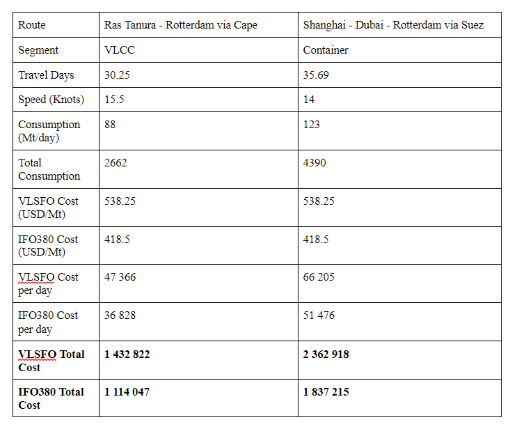
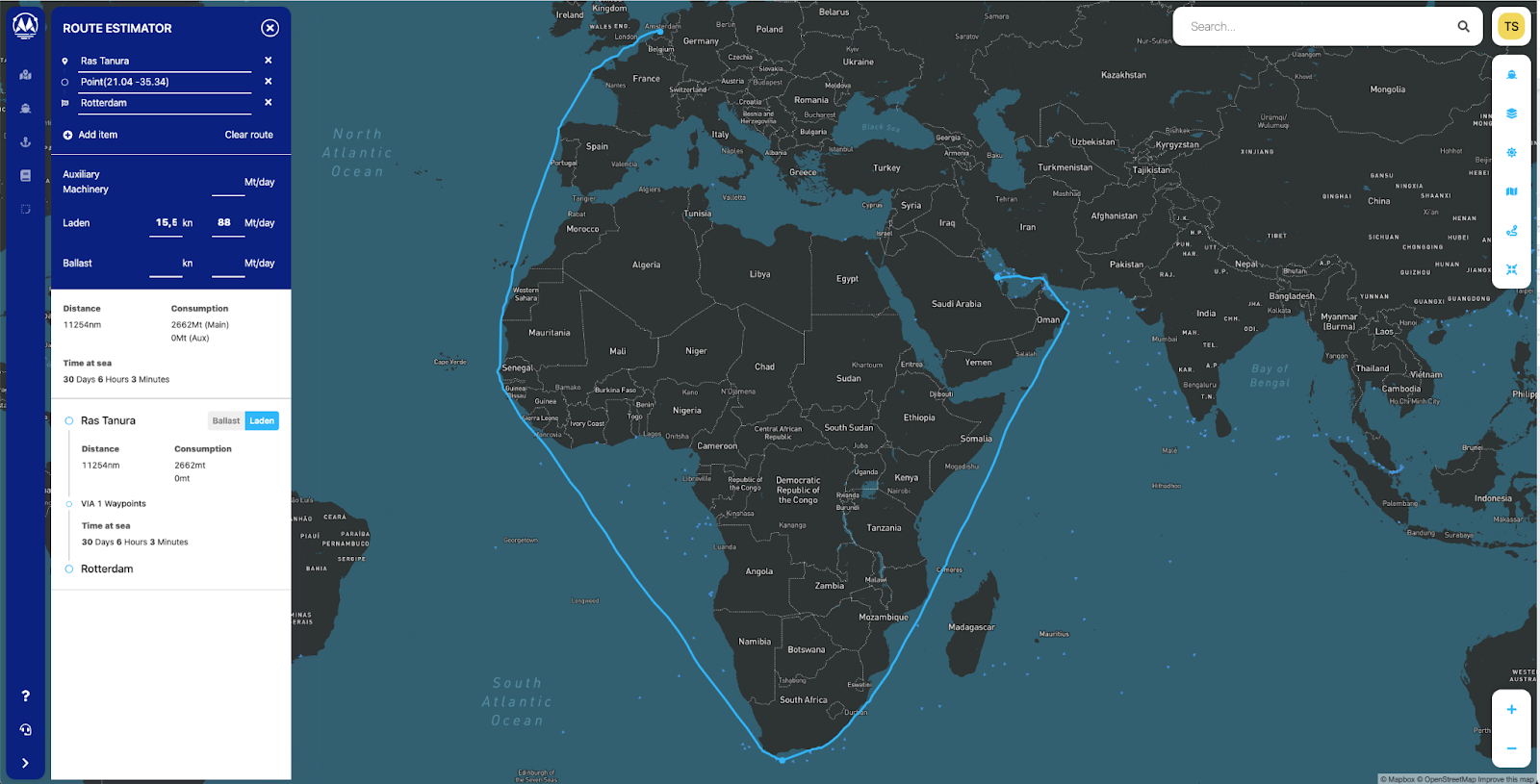
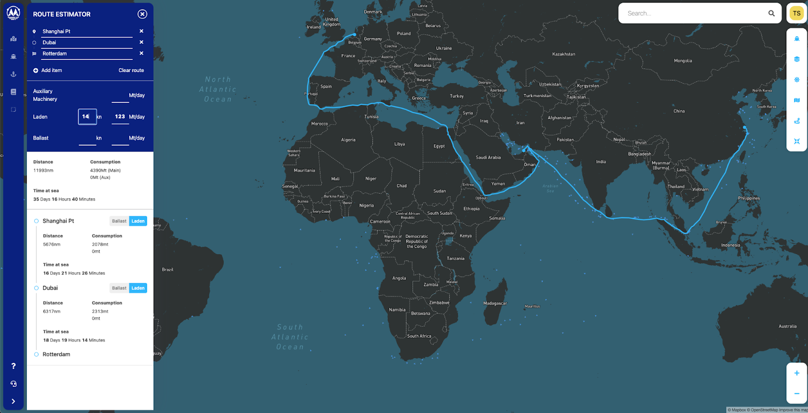
From the vessel operation side, revenue is generated by transporting cargo within the allotted time schedule. The major contributor to operating costs is bunkers, which typically makes up 50-80 % of a vessel's operating costs [4]. Using the Maritime Optima route estimator and simple back-of-the-envelope bunker calculations, we can illustrate the bunker costs for performing a voyage given VLSFO and IFO380 prices in Singapore 2021-06-22.
Therefore, operators always want to minimize fuel spending both in short and long term, given the constraint of transporting their cargo on time.
In a short-term perspective, bunker costs will be controlled by the tuning of the speed and consumption, negotiate favourable bunker clauses in the charterparties, bunker hedging or trying to optimise bunker purchase and volumes. Operators have so far not addressed the timing of purchase as a means to reduce bunker costs. However, access to reliable real-time bunker trading data from many ports simultaneously might make timing of bunker procurement more interesting as a variable to be optimized.
In a longer-term perspective new technology and software, new engine types and new types of fuel will be evaluated.
Bunker pricing curves
Oil markets have been seen as something close to perfect competition, impenetrable and prone to exogenous shocks, political, economic or other. In order to address the timing issue accurate prices are necessary. However, an accurate view of prices is not entirely easy to obtain due to the nature of how bunkers are sold and purchased. The most obvious point is that physical bunkers are not traded on an exchange, but locally in ports. It follows that the liquidity of transactions is less than desired and outside of the main hubs, such as Rotterdam and Singapore, price fluctuations in bunkers compared to oil prices can be substantial at times. Price variations for the different products can also be affected differently due to local supply and demand. Though it is important to note that the link to oil prices is invariably present through time.
In this picture, efficient use of data continues to play a vital role. Regulatory mandates enforce data collection schemes to monitor vessel emissions and potentially sanction companies not abiding to the implemented standards. Meanwhile, vessel operators focus on route optimization utilizing weather data, tide information, bunker port locations, and congestion forecasts to reduce fuel consumption. From a cost perspective, due to the highly volatile bunker prices, accurate data driven price predictions have the potential to award vessel operating companies with large savings.
A prerequisite for such predictions would be transparent historical bunker prices for the multitude of different ports providing bunker to vessels. Further, due to the increasing regulatory restrictions on particle emissions such as NOx, COx and CO2 in ports, vessel operators also need access to accurate price information for the different grades of bunker fuel such as IFO180, IFO380, MGO, ULSFO, and VLSFO.
To this end, Bunkerex Ltd. provides prices based on real stems adjusted for volume, availability, and credit. This is why we at Maritime Optima AS are proud to have partnered with BunkerEx. Their bunker price information enriches our product and forms the baseline for further data driven price predictions which will be implemented in our product.
BunkerEx Data
After loading the BunkerEx data into a Pandas DataFrame, this is what the data will look like.
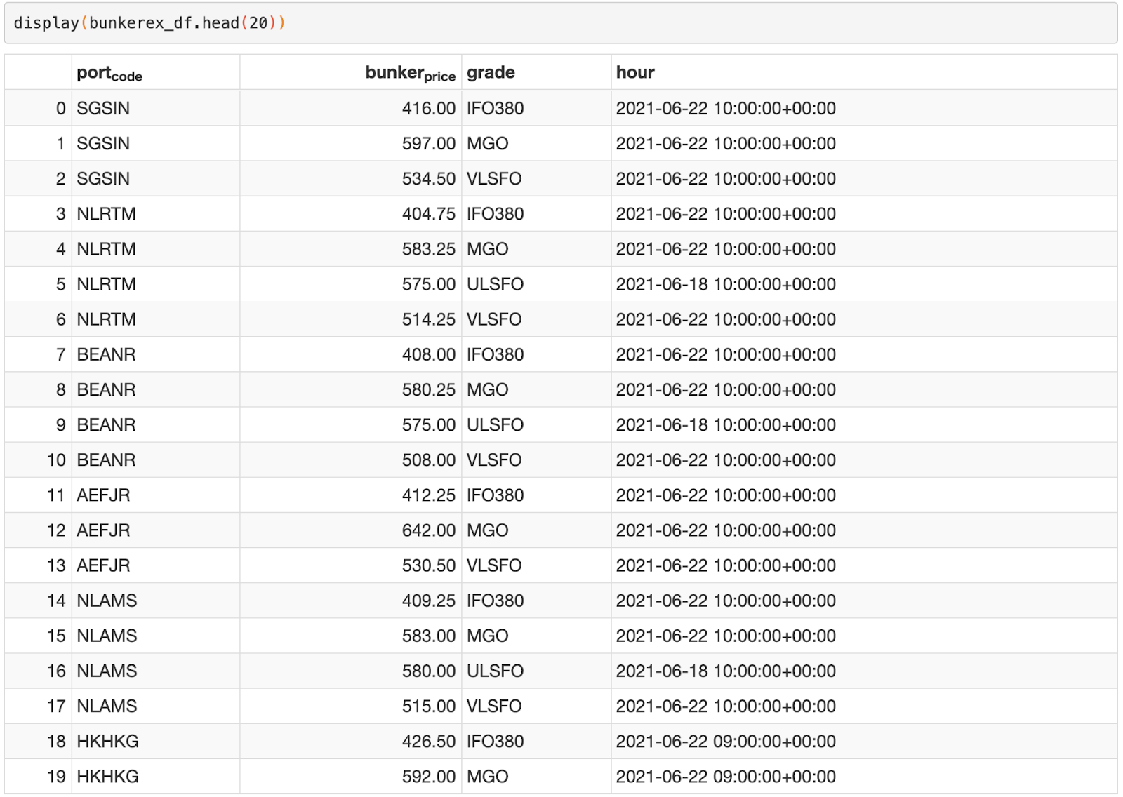
In order to further analyze the bunker price data, our main aim will be to create index prices. These prices will be aggregated on an hourly basis, and will serve to identify trends among the different ports and grades. To adjust for structural price variances, only data for the previous 6 months will be used in our analysis.
Missing Values
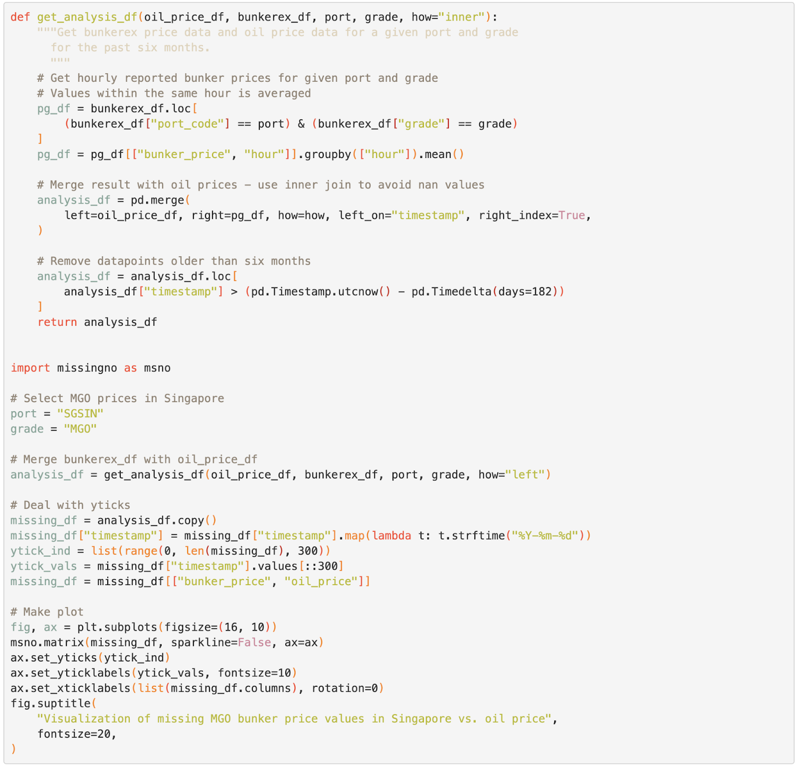
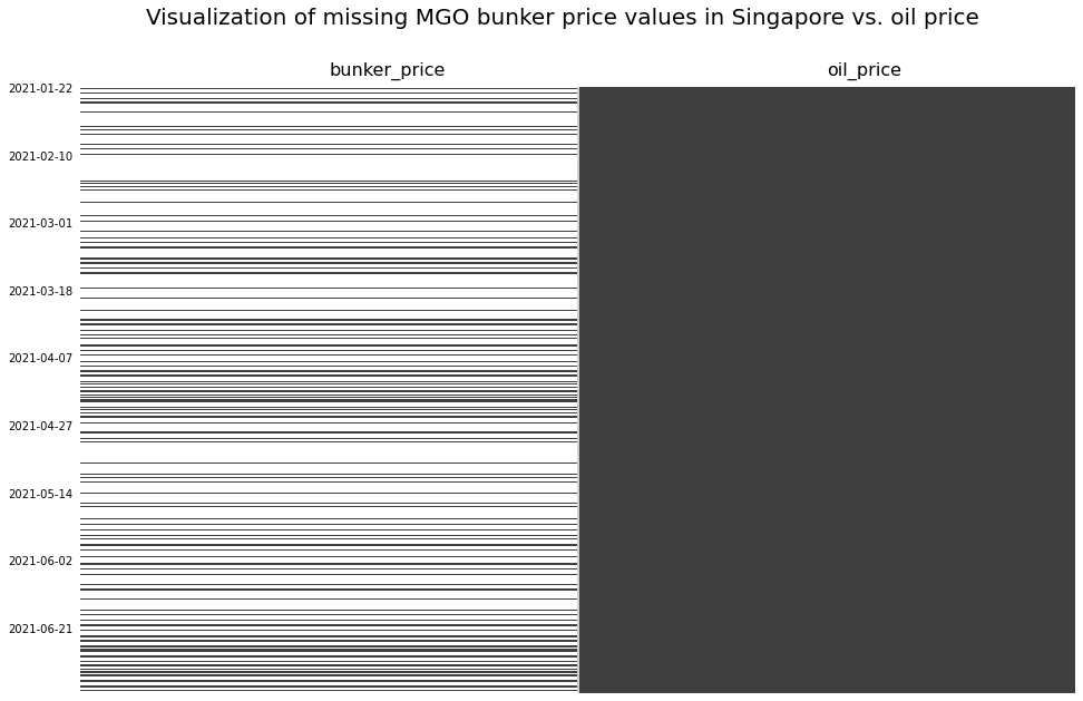
As bunker prices are not reported for port and grade on an hourly basis, missing values will have to be imputed. To visualize the number of missing values, we can utilize the excellent package missingno. We will use MGO bunker prices in the port of Singapore for our example analysis in this blog post.
Imputation by robust linear regression
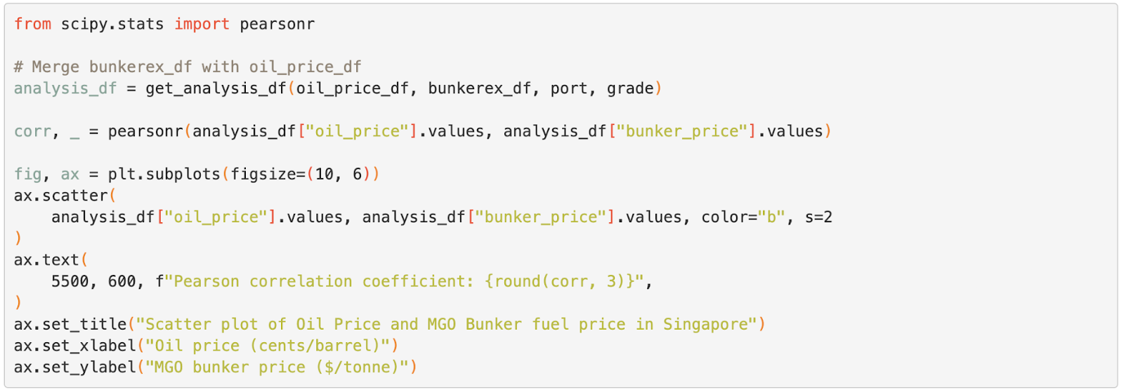
Rather than using a simple moving average or forward fill, we will take advantage of the highly correlated oil price to impute the missing values. Creating a scatter plot of oil prices and MGO bunker prices in the port of Singapore yields the following plot. The Pearson correlation coefficient is also provided.
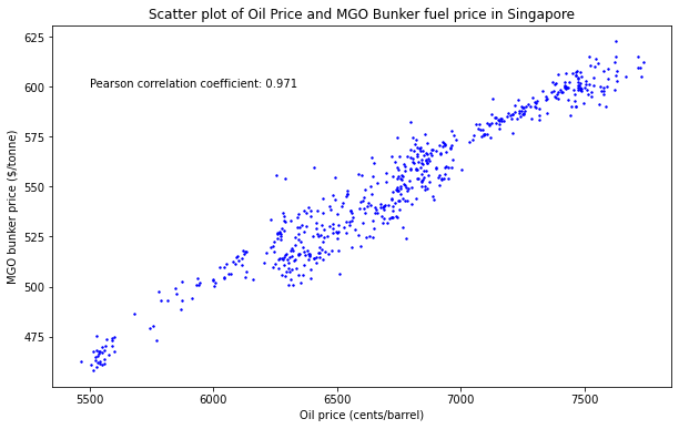
Given this information, we can utilize a simple linear regression model to estimate the missing bunker prices from above. More formally, given the \(n\) data pairs \({(x_i, y_i), i = 1, \ldots, n}\) and we want to find estimates for \(\hat y\) that minimizes the error \(\varepsilon\) in the relationship:
$$\hat y(w, x) = w_{0} + w_{1}x_1 + \varepsilon.$$
The best fit weights \(w_{0}\) and \(w_{1}\) will be the values that minimizes the
least square minimization problem:
$$\min_{w} || X w - y||_2^2$$
This approach relies on several strong assumptions such as linearity, constant variance, and independence of errors [5]. The best fit of simple linear regression may be affected when the underlying assumptions are broken. In particular, least squares estimates for linear regression models are highly sensitive to outliers. As the assumptions regarding independence of errors are not likely to hold for bunker prices of different grades and in different ports. Ordinary least squares estimates are likely to yield poor imputation estimates.
Luckily, approaches such as robust regression are available, which aim to not be overly affected by violations of assumptions by the underlying data-generating process [6]. One such approach is a robust hybrid of lasso and ridge regression called the Huber regression [7].
Ridge regression minimizes the loss function given by:
$$\min_{w} || X w - y||_2^2 + \alpha ||w||_2^2,$$
which extends the squared error loss function by introducing a penalty on the size of the weights with \(\alpha > 1\) being a complexity parameter controlling the amount of shrinkage.
Huber regression, further extends ridge regression by making use of the Huber loss and thus aims to minimize the loss function given by:
$$\min_{w, \sigma} {\sum_{i=1}^n\left(\sigma + H_{\epsilon}\left(\frac{X_{i}w - y_{i}}{\sigma}\right)\sigma\right) + \alpha {||w||_2}^2}$$
where:
$$\begin{split}H_{\epsilon}(z) = \begin{cases} z^2, & \text {if } |z| < \epsilon, \\ 2\epsilon|z| - \epsilon^2, & \text{otherwise} \end{cases}\end{split}.$$
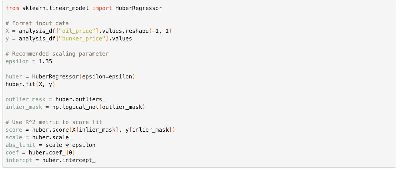
Huber regression differs from ridge regression in the way that it applies a linear loss to samples that are classified as outliers. A sample is classified as an inlier if the absolute error of the sample is less than some threshold [8]. Errors smaller than \(\epsilon\sigma\) get squared while larger errors increase the criterion only linearly. Huber recommends an \(\epsilon\) value of 1.35 as it retains 95% statistical efficiency for normally distributed data [7].
Plotting the Results
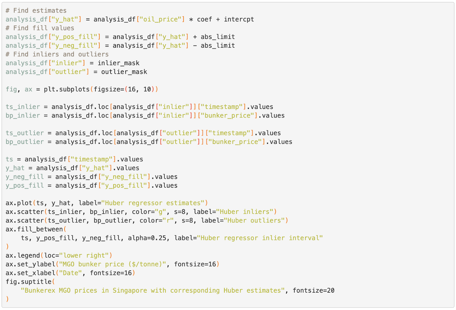
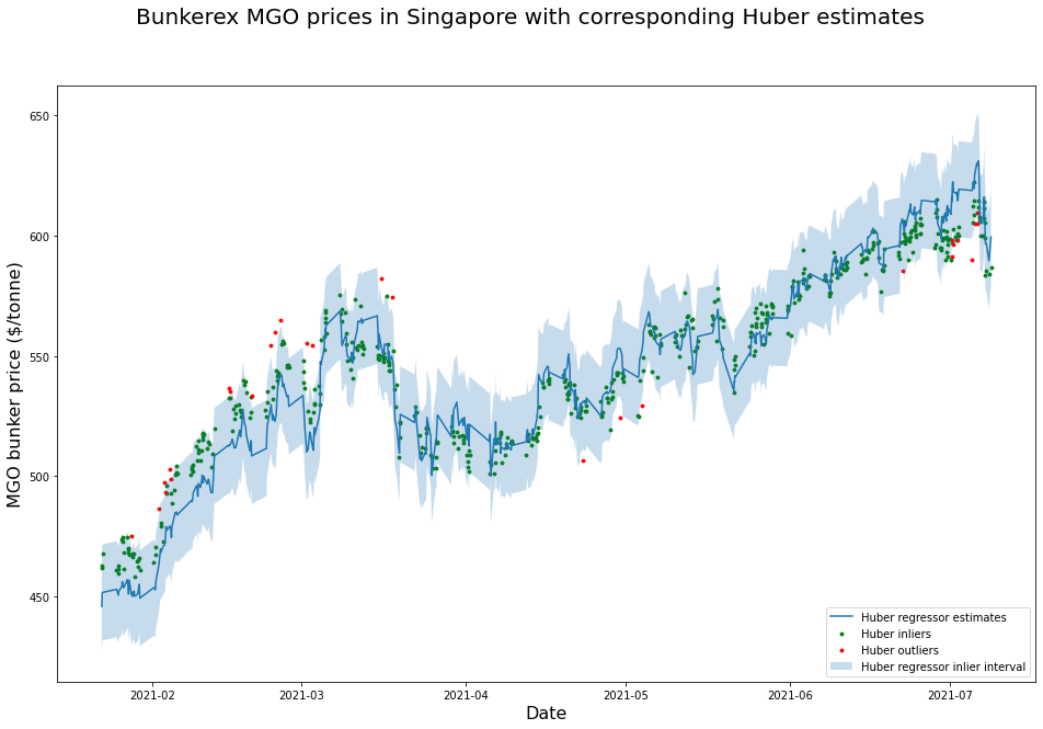
After having fitted the data, let us plot the inlier, outliers and the best fit curve.
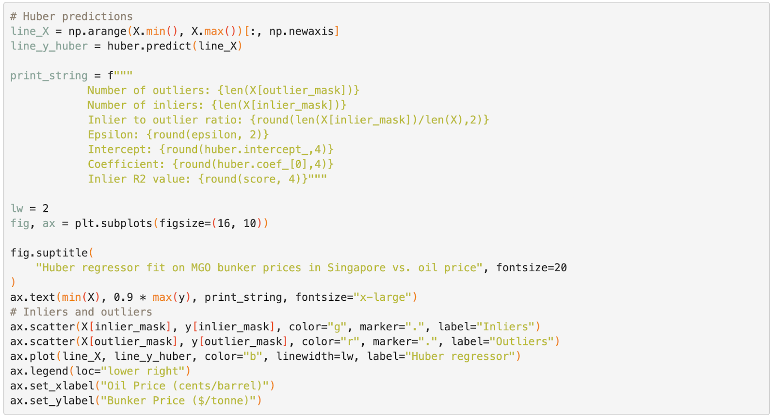
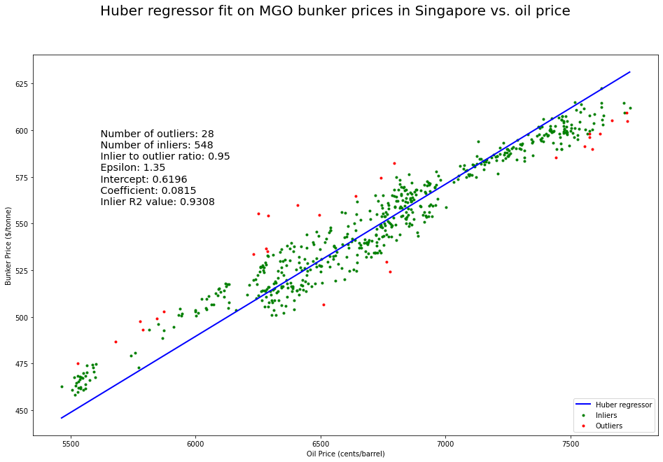
Finally, we can plot the original BunkerEx MGO bunker prices in Singapore along with the outlier decision boundary and Huber estimates.
Conclusion
BunkerEx provides transparent historical bunker prices for many different ports and grades. In order to provide meaningful bunker price predictions in the future, it is helpful to estimate historical prices. In this blog post we have seen how one can make use of robust regressors to estimate hourly bunker index prices. This will be a helpful starting point for future work with bunker optimizing along a route, bunker forecasting and pre calculation.
References
[1] I. T. Forum, ITF Transport Outlook 2017. 2017.
[2] S. Singh and B. Sengupta, Sustainable Maritime Transport and Maritime Informatics, pp. 81–95. Progress in IS, Springer International Publishing, 2020.
[3] T. Smith, J. Jalkanen, B. Anderson, J. Corbett, J. Faber, S. Hanayama, E. O’Keeffe, S. Parker, L. Johansson, L. Aldous, C. Raucci, M. Traut, S. Ettinger, D. Nelissen, D. Lee, S. Ng, A. Agrawal, J. Winebrake, M. Hoen, and A. Pandey, Third IMO GHG Study 2014: Executive Summary and Final Report. 07 2014.
[4] I. Hemnani, “Bunker Planning Optimisation Problem,” Nov. 2018.
[5] “Linear regression - Wikipedia.” https://en.wikipedia.org/wiki/Linear_ regression#Assumptions
[6] “Robust regression - Wikipedia.” https://en.wikipedia.org/wiki/ Robust_regression
[7] A. B. Owen, “A robust hybrid of lasso and ridge regression,” tech. rep., 2006.
[8] “1.1. Linear Models — scikit-learn 0.24.2 documentation.” https://scikitlearn.org/stable/modules/linear _model.html#robustness-regression- outliers-and-modeling-errors


